Tech Blog
Getting explainability right part 2: Beware of approximations

This is the second blog post in a three-part series on getting explainability right. In the previous post, we showed how to decide between using interpretable models or black box explainability. We concluded that there are many situations that require more complex models and therefore necessitate black box explainability. In this blog post, we’ll discuss the danger of inappropriate approximations for black box explainability.
Black box explainability is hard. Even seemingly simple information about any model, such as the importance of each feature, is very complicated and expensive to calculate correctly.
In order to simplify the calculation, it’s common to make two approximations: linearity and feature independence. Popular methods which make these assumptions include LIME (local linear approximation, feature independence), SHAP (feature independence), TreeSHAP (a modified version of feature independence), and DeepLIFT/DeepSHAP (linearity and feature independence). As we will demonstrate in this blog post, both these approximations are problematic and can lead to misleading explanations.
Approximations themselves aren’t a problem per se; in other fields, like physics, they are commonly used to describe everything from small oscillations of a pendulum to the propagation of gravitational waves through the universe. However, physicists are careful to track the size of the error caused by the approximation and check that it is small. We must do the same in explainability: if we do not know how good an approximation is, we shouldn’t make it.
In the remainder of this blog post, we’ll investigate the quality of approximations in black-box explainability – and when those approximations can cause serious problems.
(Local) linearity
LIME is the most popular method to use linear approximations. LIME constructs a weighted linear approximation to the model, with a weighting kernel that is large around the data point for which we would like to explain the model, and decays rapidly away from this data point (see figure 3 in the LIME paper). This is a delicate balance: if the approximation isn’t local enough, it might miss important aspects of the model. If it’s too local, it might exaggerate unimportant irregularities in the model output. In practice, this can make it hard to ensure that explanations with LIME are faithful without investigating the results in great detail.
Even in the simplest situations, a linear approximation misses interactions between features.
Let’s say we are trying to predict failure rate in a factory machine. We consider three features for this problem:
• The status of the generator.
• The status of the backup generator.
• An aggregated feature that defines if there are faults with any other components associated with the machine.
The machine is guaranteed to fail in the rare event that both the generator and its back-up have failed. Failure in the aggregated (third) feature occurs more often, but does not always result in the machine failing.
Since LIME makes a linear approximation, it cannot take this interaction between features into account, so it underestimates the impact of the generator and its back-up on the model outcome (see Fig. 1). In real life, such errors could lead to expensive misidentification of systematic faults.
This toy example is so simple that we should have used an interpretable model in the first place. More complex situations that require black box models often also have more complex interactions of features, making LIME’s explanations even less trustworthy.
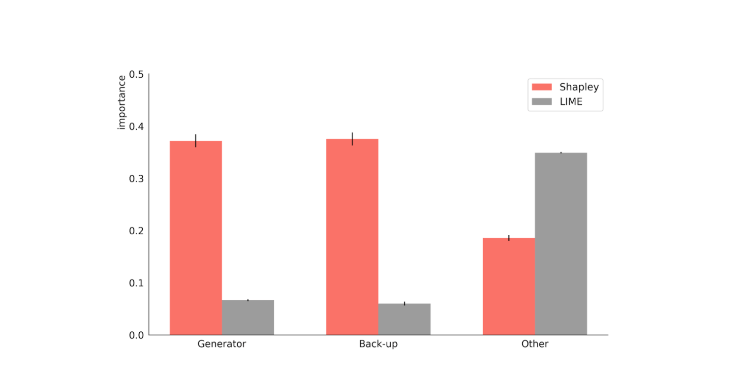
Fig. 1: LIME and Shapley explanations for a model trained on a toy dataset of machine failure caused by simultaneous failure in the generator and back-up generator or failure in any other component. This is a local explanation for an instance when all three components failed. LIME makes a linear approximation, Shapley does not.
Feature independence
Explanations based on Shapley values usually don’t assume linearity and do take interactions of features into account, making them much more reliable – in principle.
However, both LIME and Shapley values require drawing fabricated data points from the data distribution (see our previous blog post). To achieve this, all public implementations to date assume that the features are independent of each other. Of course, for real-world data this is rarely the case, so we know that this assumption is incorrect, but how much does this affect the explanations?
To investigate this, let’s compare Shapley values, calculated with an implementation that assumes feature independence and a new method we proposed in a recent paper that does not. We’ll use the public 1994 US census as our dataset, with a model trained to predict income.
If we ignore how features like marital and relationship status, education, occupation, or age relate to each other in census data, we can run into significant problems. When we construct fabricated data points to calculate Shapley values or LIME coefficients, we might get unrealistic data points, such as a 17 year-old married single person who holds a doctorate degree.
Using model predictions on bogus data points like these for the model explanation will give us bogus results. Furthermore, if we assume feature independence, the explanations cannot reflect how the model works on the data in practice. For example, they might lead us to believe that the model does not use information about a person’s relationship status even though it picks up most of this information from correlations with other features, like marital status.
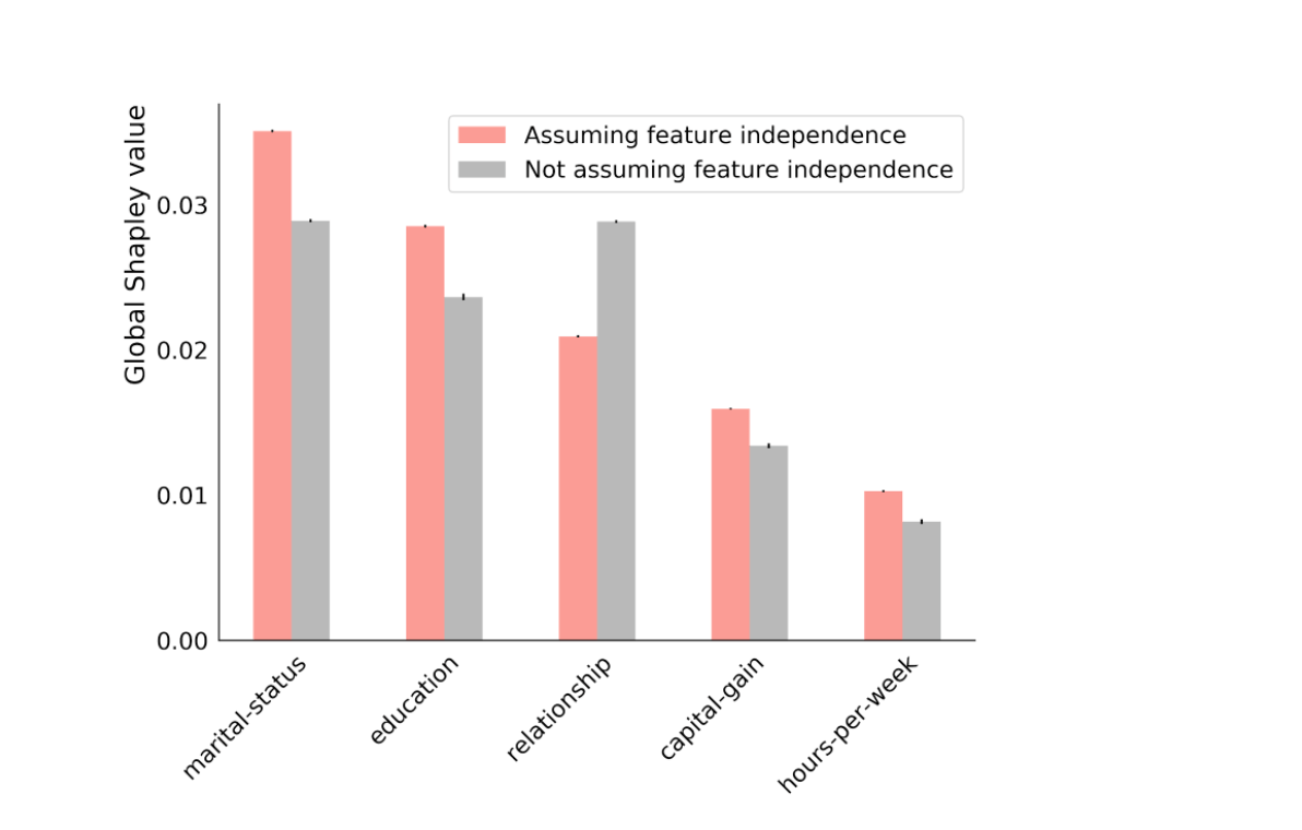
Fig. 2: Five largest global Shapley values for a model predicting income in the open-source US census data. Assuming feature independence overstates the importance of marital status compared to relationship. This effect can be even more extreme for local Shapley values.
The results in Fig. 2 clearly show this effect: in the original implementation, which assumes feature independence (coral), the marital status and relationship features have very different contributions to the explanation, despite being highly correlated. If we assume that features may be dependent (grey bar in Fig. 2), these two features are correctly assigned equal importance in the explanation. The figure shows the global Shapley values: the errors in the explanations for a particular individual can be much more extreme.
It’s clear that the feature independence assumption can lead to wrong or misleading model explanations. In general, we have no way to estimate the effect of this assumption, so we prefer not to make it in our work.
In the next blog post, we will outline how Shapley values can be calculated without making unjustifiable assumptions (while still keeping the runtime reasonable). Furthermore, we will outline the method we propose at Faculty for taking causality into account.